#select TX state only given it has 99% of the data points
injuries %>%
  filter(st == "TX") -> injuries

#factor gender as M anf F using dplyr case_when and drop NAs
injuries <- injuries %>%
  mutate(gender = case_when(
    gender %in% c("F", "f") ~ "F",
    gender %in% c("M", "m") ~ "M")
        ) %>%
  drop_na(gender)

#convert age to numeric and drop nas

injuries <- injuries %>%
  mutate(age=as.numeric(age)) %>%
  filter(!is.na(age))

## Warning: NAs introduced by coercion

#convert the excel numeric data format using janitor package

injuries$date_inj_excel <- excel_numeric_to_date(as.numeric(as.character(injuries$injury_date)))

## Warning in
## excel_numeric_to_date(as.numeric(as.character(injuries$injury_date))): NAs
## introduced by coercion

#convert the dates to numeric using the lubridate package
  
injuries$date_inj <- parse_date_time(injuries$injury_date, orders = c("mdy"))

## Warning: 306 failed to parse.

#combine the two columns

injuries %>%
  unite("date_final", date_inj:date_inj_excel) -> injuries 

#remove the NA_ and _NA #using regexprs 

injuries$datefinal <- sapply(injuries$date_final, function(x) gsub("NA_", "", x))
injuries$datefinal <- sapply(injuries$datefinal, function(x) gsub("_NA", "", x))

#parse as date
injuries$datefinal <- parse_date(injuries$datefinal) 

#include year and month 
injuries %>%  
  mutate(year= lubridate::year(datefinal),
         month = lubridate::month(datefinal)
  ) -> injuries

Data Viz

Here we determine how many injuries were recorded per month and per year. To analyse which months need extra attention because we expect more injurries in the park during summer compared to winter.

#injuries per year
injuries %>%
  group_by(year) %>%
  tally() %>%
  ungroup() %>%
  drop_na() %>%
  ggplot(injuries, mapping=aes(reorder(year, -n), n , fill=year, label=n))+
    geom_col(show.legend = FALSE) +
    geom_text(nudge_y = 10) +
    labs(title= " Amusement Park Injuries per Year", 
       caption = "By am_innocenter for #TidyTuesdy \n Data source : data.world", x= " Year", y="Number of Injuries" )+
  theme(panel.background = element_rect(fill="bisque")) + #, colour = "#6D9EC1")) +
  theme(text = element_text(family = "Comic Sans MS", size = 14),
        plot.caption = element_text( size=10, color = "grey40"),
        plot.title =element_text(size = 16, face="bold", vjust=1) )+
  theme(
    # Hide panel borders and remove grid lines
    panel.border = element_blank(),
    panel.grid.major = element_blank(),
    panel.grid.minor = element_blank()        ) +
  theme(legend.position = "none")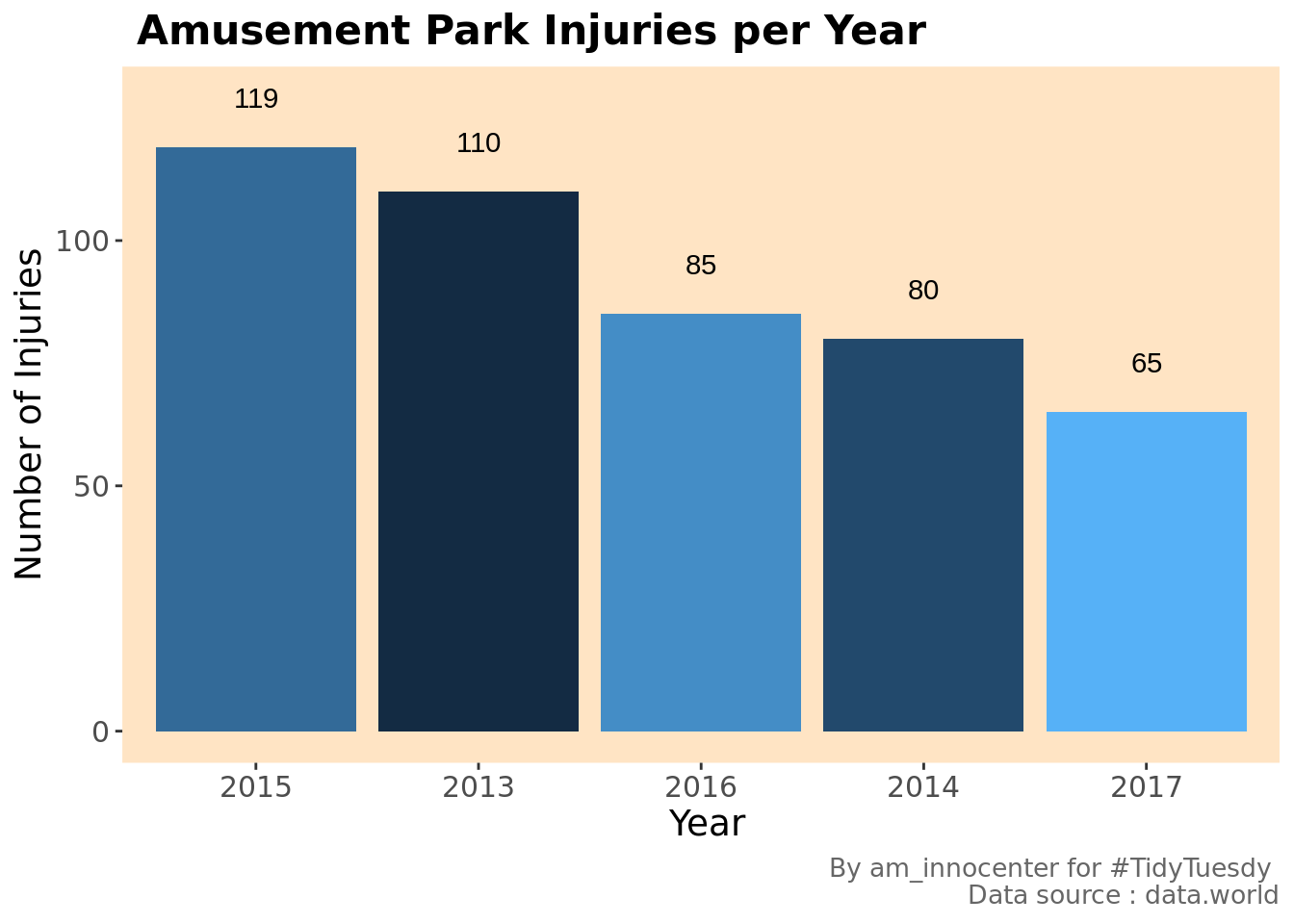

The numer of injuries over the years have been decreasing significantly. This could be to a number of reasons. To speculate the least we are getting better at control measures on the parks to avoid injuries.

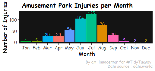
To answer how many injuries were recorded per month we utilized the month.abb built-in constant to rearrange months from Jan - Dec

#injuries per month

injuries %>%
  group_by(Months=month.abb[month]) %>% #built-in constant month.abb has 3-letter abbrev for the months
  tally() %>%
  ungroup() %>%
  drop_na() %>%
  ggplot(injuries, mapping=aes(Months, n , fill=Months, color=Months, label = n))+
    geom_col(show.legend = FALSE)  +
    geom_text(nudge_y = 6) +
    scale_x_discrete(limits= month.abb) + #rearranges the month order
    labs(title= " Amusement Park Injuries per Month", 
         caption = "By am_innocenter for #TidyTuesdy \n Data source : data.world", x= " Month", y="Number of Injuries"
         )+
    theme(panel.background = element_rect(fill="gray8")) + #, colour = "#6D9EC1")) +
    theme(text = element_text(family = "Comic Sans MS", size = 14),
          plot.caption = element_text( size=10, color = "grey40"),
          plot.title =element_text(size = 16, face="bold", vjust=1) )+
    theme(
    # Hide panel borders and remove grid lines
    panel.border = element_blank(),
    panel.grid.major = element_blank(),
    panel.grid.minor = element_blank()        ) +
    theme(legend.position = "none")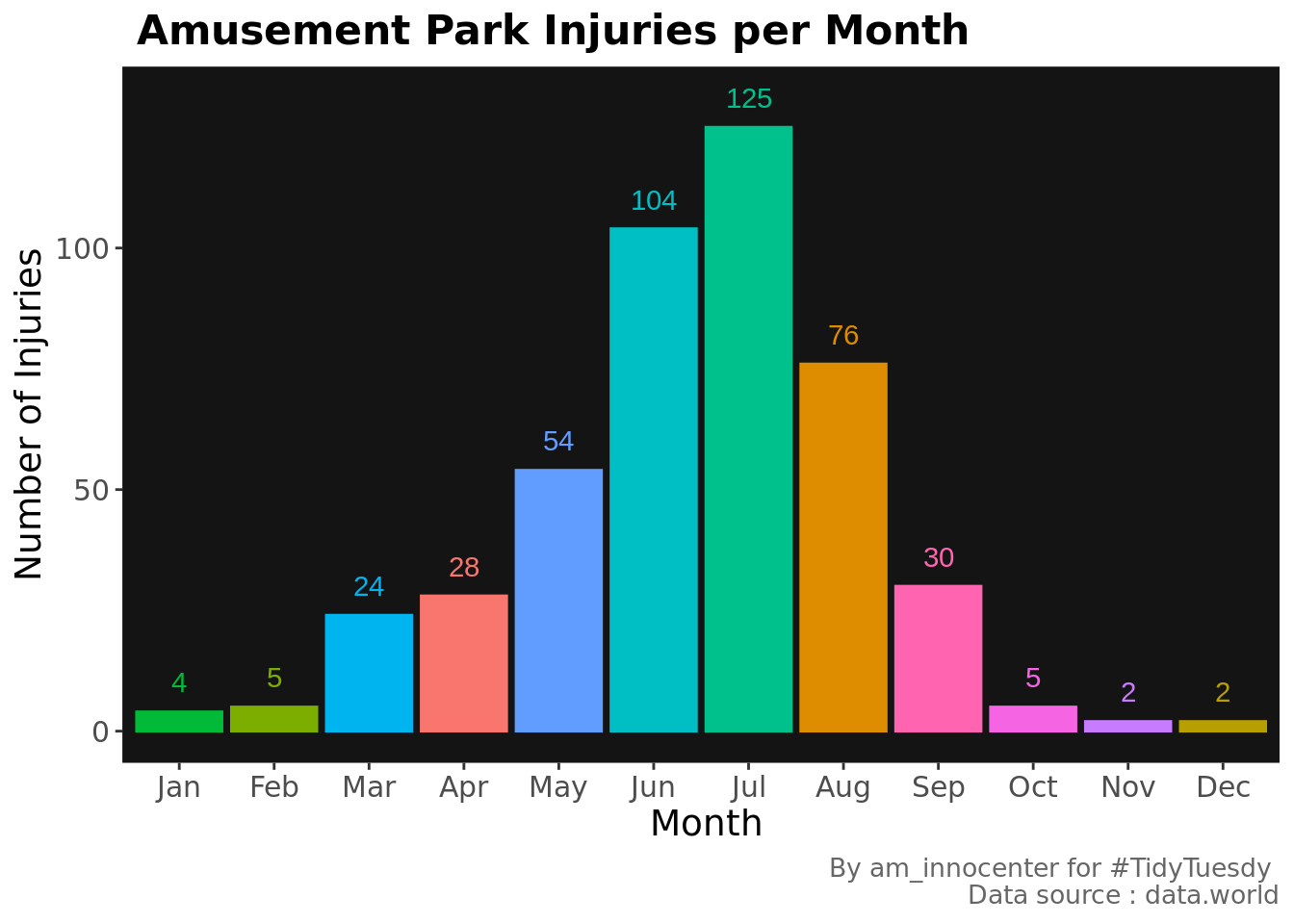

As we had pre-empted, June-Aug has the highest number of injuries.

Who got injured more? Male or female? children or adults?

injuries %>%
  select(gender,age) %>%
  filter(age>=0) %>%
  mutate(age_bins = cut_interval(age,7)) %>%
  group_by(gender, age_bins) %>%
  tally() %>%
  ungroup() %>%
  mutate(count= if_else(gender=="F", -n, n)) %>%
  ggplot(aes(x=age_bins, count , fill=gender))+
    geom_bar(stat = "identity", show.legend = FALSE) +
    coord_flip()+
    scale_y_continuous(breaks = seq(-60, 60, 20),
                       labels = c(seq(60,0,-20), seq(20,60,20)))+ #renaming y aesthetics
  labs(title= "Amusement Park injuries per Age and Gender",
       x="Age Group", y="Number of Injuries",
       caption = "Plot by @am_innocenter for #TidyTuesday \n Data source: data.world")+
  theme_minimal()+
  theme(text = element_text(family = "Comic Sans MS", size = 14),
        plot.caption = element_text( size=10, color = "gray40"),
        plot.title =element_text(size = 16, face="bold", vjust=1) ) +
  geom_text(aes(5,-60), label="\u2640", hjust = 0.5, size = 25,color = "#F8766D", family = "Comic Sans MS") +
  geom_text(aes(5,45), label="\u2642", hjust = 0.5, size = 25, color = "#00BFC4", family = "Comic Sans MS")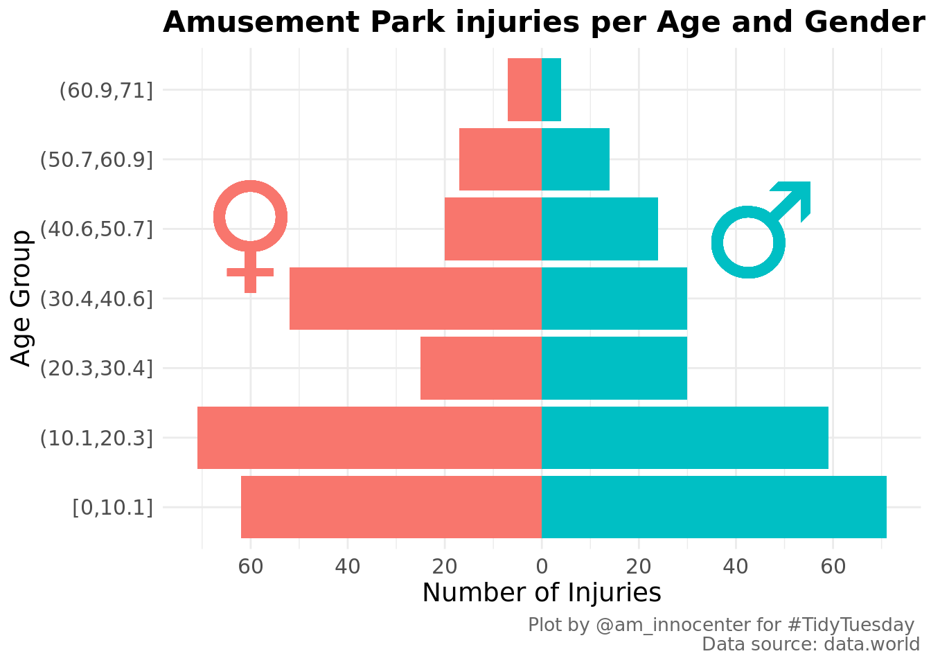 

Trick I learned to pick the colors use ggplot_build(plotname).

Children reported more injuries compared to adults. Females are slightly more by 5% compared to the males.

Analyse the cause of injuries and body parts affected below using tidytext.

injuries %>%
  select(gender,age , body_part) %>%
  mutate(age_bins = cut_interval(age,7)) %>%
  count(body_part,age_bins, sort = TRUE) %>%
  top_n(20) %>%
    ggplot(aes(age_bins,n, fill=body_part)) +
    geom_col() +
    coord_flip() +
    theme_minimal()+
    labs(title= " Amusement Park Injuries", subtitle = "Body parts injured per age group", 
         caption = "By am_innocenter for #TidyTuesdy \n Data source : data.world", x= " Age Group", y="Number of Injuries" )+
    theme(panel.background = element_rect(color="grey40")) +
    theme(text = element_text(family = "Comic Sans MS", size = 14),
        plot.caption = element_text( size=10, color = "grey40"),
        plot.title =element_text(size = 16, face="bold", vjust=1) ) +
    theme(legend.position = c(.97, .97),legend.justification = c("right", "top"),
          legend.box.just = "right", 
          legend.box.background = element_rect(fill="grey80", color="grey40")) 

## Selecting by n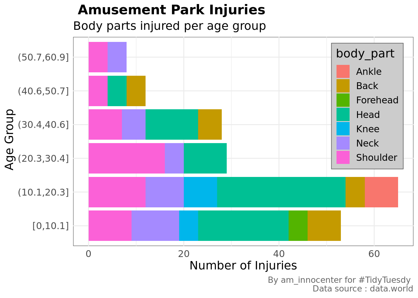

The most injured parts are head and shoulder among children and teenagers. For the elderly > 50 years it is the neck and shoulder. Most adults will be in the park taking care of the younger ones - the most injured body parts are shoulder and head.

injuries %>%
  select(cause_of_injury) %>%
  unnest_tokens(word, cause_of_injury) %>%
  anti_join(stop_words, by="word") %>%
  count(word, sort = TRUE) %>%
  ungroup() %>%
  filter(n > 20) %>%
  ggplot(mapping=aes(reorder(word,n), n, fill=n, label=n))+
    geom_col()+
    geom_text(nudge_y = 2) +
    coord_flip() +
    labs(title= " Amusement Park Injuries", 
         subtitle = "Top Words in Cause of Injury", 
         caption = "By am_innocenter for #TidyTuesdy \n Data source : data.world", 
         x= " Words in Cause", y="Count")+
    theme(panel.background = element_rect(fill="beige")) + 
    theme(text = element_text(family = "Comic Sans MS", size = 14),
          plot.caption = element_text( size=10, color = "grey"),
          plot.title =element_text(size = 16, face="bold", vjust=1) )+
    theme(
      # Hide panel borders and remove grid lines
      panel.border = element_blank(),
      panel.grid.major = element_blank(),
      panel.grid.minor = element_blank()        ) +
    theme(legend.position = "none")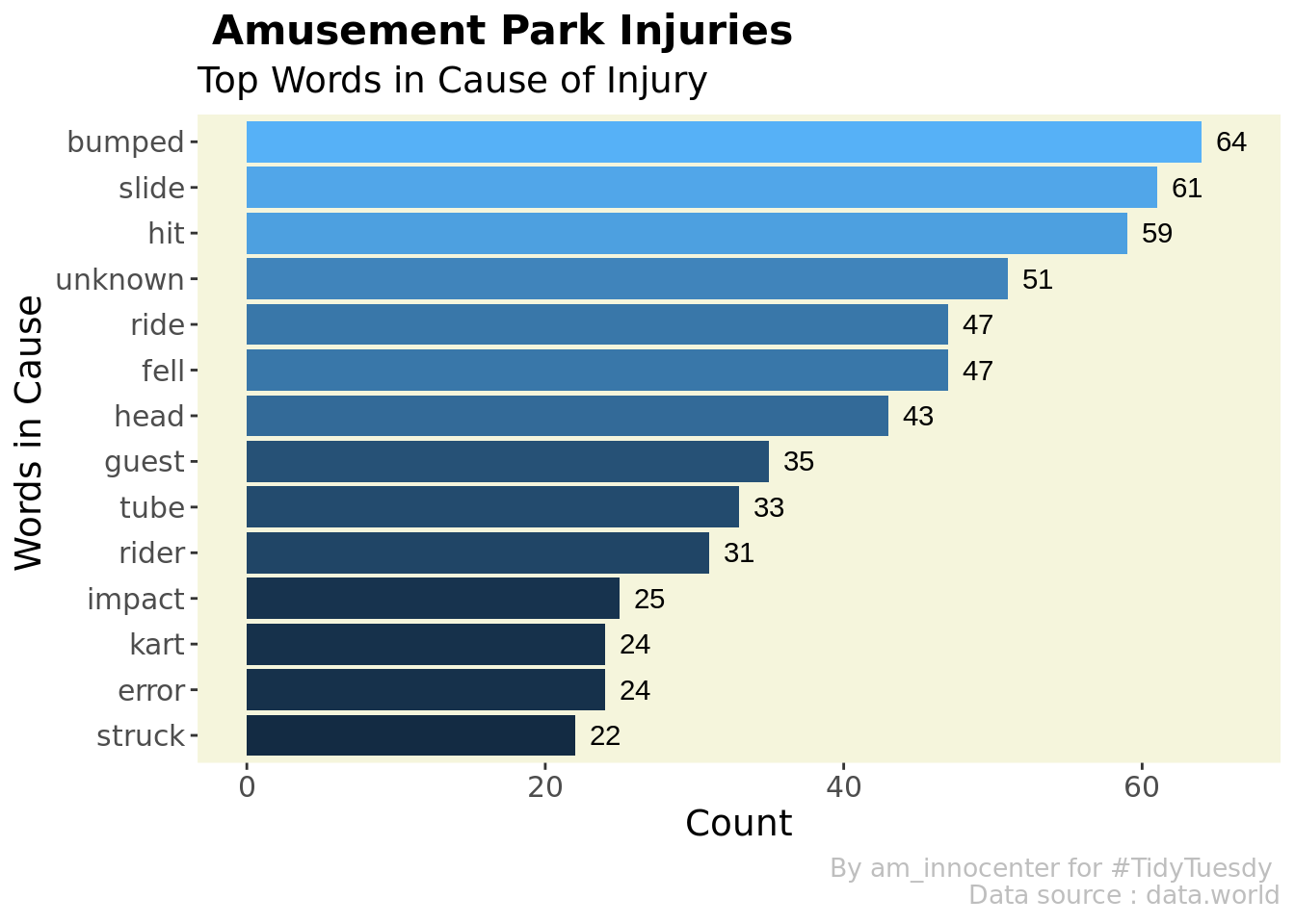

I wanted to determine the words that occur commonly in pairs and how often sequence of word1 and word 2 occurs

#ngrams
injuries %>%
  unnest_tokens(biwords, body_part, token="ngrams", n=2) %>%
  count(biwords, sort=TRUE) %>%
  top_n(15) %>%
  filter(!is.na(biwords)) %>%
  ggplot(aes(reorder(biwords,n),n, fill= n, label=n))  +
    geom_col(show.legend = FALSE)+
    coord_flip() +
    geom_text(nudge_y = 0.5)+
    labs(title= "Amusement Park injuries", subtitle = "Most words occuring together",
       x="Bi-words ", y="Count",
       caption = "Plot by @am_innocenter for #TidyTuesday \n Data source: data.world") +
    theme(panel.background = element_rect(fill="beige")) + 
    theme(text = element_text(family = "Comic Sans MS", size = 14),
          plot.caption = element_text( size=10, color = "grey"),
          plot.title =element_text(size = 16, face="bold", vjust=1) )+
    theme(
      # Hide panel borders and remove grid lines
      panel.border = element_blank(),
      panel.grid.major = element_blank(),
      panel.grid.minor = element_blank()        ) +
    theme(legend.position = "none")

## Selecting by n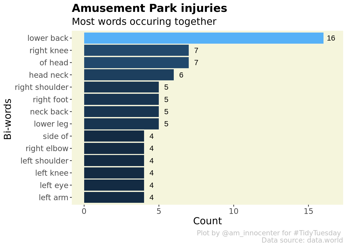

#Learnings

Converting excel numeric date format. Using tidytext, discovering janitor package,

In case you have feedback, questions, suggestions do not hesitate to leave a comment.