Understanding US Student Loan debt

November 26, 2019

This week the data was inspired from the Dignity & Debt project. This will help in understanding and spreading awareness around Student Loan debt. The data source is here

The objective for this is to perform data visualization and determine the most preferred method of payment for student loans in the US. I will use patchwork package to combine plots.

Loading the data

loans <- read.csv("https://raw.githubusercontent.com/rfordatascience/tidytuesday/master/data/2019/2019-11-26/loans.csv")

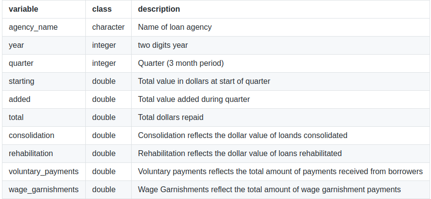
glimpse(loans)

## Observations: 291
## Variables: 10
## $ agency_name        <fct> "Account Control Technology, Inc.", "Allied Inters…
## $ year               <int> 15, 15, 15, 15, 15, 15, 15, 15, 15, 15, 15, 15, 15…
## $ quarter            <int> 4, 4, 4, 4, 4, 4, 4, 4, 4, 4, 4, 4, 4, 4, 4, 4, 4,…
## $ starting           <dbl> 5807704381, 3693337631, 2364391549, 704216670, 295…
## $ added              <dbl> 1040570567, NA, NA, NA, NA, NA, 1040946705, NA, NA…
## $ total              <dbl> 122602641.8, 113326847.1, 83853003.0, 99643903.3, …
## $ consolidation      <dbl> 20081893.9, 11533808.6, 7377702.9, 3401361.4, 8946…
## $ rehabilitation     <dbl> 90952573, 86967994, 64227391, 85960328, 58395653, …
## $ voluntary_payments <dbl> 5485506.86, 4885225.08, 3939866.10, 2508999.62, 29…
## $ wage_garnishments  <dbl> 6082668.43, 9939819.25, 8308043.15, 7773214.04, 54…

Original data file can be accessed through the weekly TidyTuesday Github reporsitory in this link and data source is here

Renaming columns

loans %>% 
  mutate(year = case_when(year == 15 ~ 2015, 
                          year == 16 ~ 2016,
                          year == 17 ~ 2017,
                          year == 18 ~ 2018)) -> loans

loans %>%
  group_by(year) %>%
  summarise(Total.starting = sum(starting, na.rm=TRUE)/10^9,
            Total.added = sum(added, na.rm = TRUE)/10^9,
            Total.repaid = sum(total, na.rm=TRUE)/10^9,
            consolidation.pay = sum(consolidation, na.rm = TRUE)/10^9,
            rehabilitation.pay = sum(rehabilitation, na.rm = TRUE)/10^9,
            voluntary.pay = sum(voluntary_payments, na.rm=TRUE)/10^9,
            wagegarnishment.pay =sum(wage_garnishments, na.rm = TRUE)/10^9 ) %>%
  arrange(desc(year))  %>%
  ungroup() -> payment.summary

loan1 <- payment.summary %>% 
  pivot_longer(starts_with("Total"), names_to = "status", values_to = "totals")  %>% 
  mutate(label = if_else(year == max(year), as.character(status), NA_character_)) %>% 
  ggplot(mapping = aes(year, totals, col=status)) +
    geom_line(show.legend = FALSE)+
    scale_color_discrete(guide = FALSE) +
    theme_classic() +
  labs(title= "Loan Amounts per Year",
       x= "Year", y="Amount in USD (billion)", caption = "By am_innocenter for #TidyTuesdy 26.11.2019 \n Data source : studentaid.ed.gov")+
  geom_label_repel(aes(label=label),nudge_x = 1, na.rm = TRUE )+
  theme(panel.background = element_rect(fill="gray8")) + #, colour = "#6D9EC1")) +
  theme(text = element_text(family = "Impact", size = 12),
        plot.caption = element_text( size=10, color = "grey40"),
        plot.title =element_text(size = 14, face="bold") )

loan2  <-  payment.summary %>% 
  pivot_longer(starts_with("Total"), names_to = "status", values_to = "totals")  %>% 
  mutate(label = if_else(year == max(year), as.character(status), NA_character_)) %>% 
  ggplot(mapping = aes(year, totals, col=status)) +
    geom_line(show.legend = FALSE)+
    scale_color_discrete(guide = FALSE) +
    scale_y_log10() +
    theme_classic() +
    labs(title= "Loan Amounts per Year", 
       caption = "By am_innocenter for #TidyTuesdy 26.11.2019 \n Data source : studentaid.ed.gov", 
       x= "Year", y="Log 10 of Amount in USD (billion)"
    )+
    geom_label_repel(aes(label=label),nudge_x = 1, na.rm = TRUE )+
    theme(panel.background = element_rect(fill="gray8")) + #, colour = "#6D9EC1")) +
    theme(text = element_text(family = "Impact", size = 12),
      plot.caption = element_text( size=10, color = "grey40"),
        plot.title =element_text(size = 14, face="bold") )

loan1 + loan2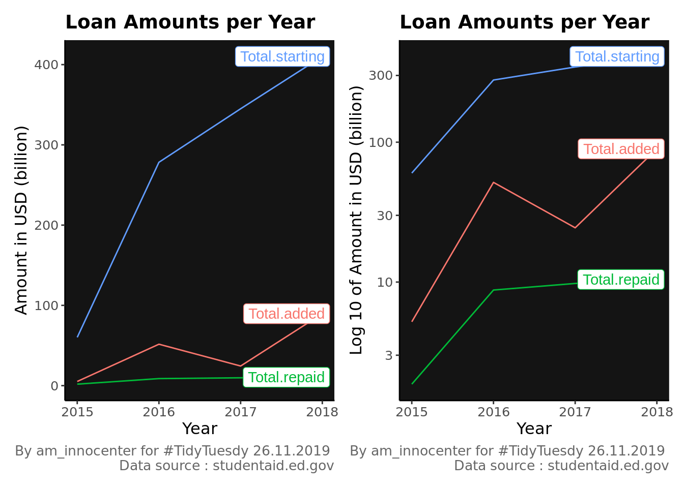

payment1 <- payment.summary %>% 
  pivot_longer(ends_with("pay"), names_to = "Method", values_to = "Payment")   %>% 
  mutate(label = if_else(year == max(year), as.character(Method), NA_character_)) %>% 
  ggplot(mapping = aes(year, Payment, col=Method)) +
  geom_line(show.legend = FALSE) +
  scale_color_discrete(guide = FALSE) +
  theme_classic() +
  labs(title= "Payment Methods & Amount Paid per Year",
       x= "Year", y="Amount in USD (billion)", caption = "By am_innocenter for #TidyTuesdy 26.11.2019 \n Data source : studentaid.ed.gov")+
  geom_label_repel(aes(label=label),nudge_x = 2, na.rm = TRUE )+
  theme(panel.background = element_rect(fill="gray8")) + #, colour = "#6D9EC1")) +
  theme(text = element_text(family = "Impact", size = 12),
        plot.caption = element_text( size=10, color = "grey40"),
        plot.title =element_text(size = 14, face="bold") )

payment2 <- payment.summary %>% 
  pivot_longer(ends_with("pay"), names_to = "Method", values_to = "Payment")   %>% 
  mutate(label = if_else(year == max(year), as.character(Method), NA_character_)) %>% 
  ggplot(mapping = aes(year, Payment, col=Method)) +
  geom_line(show.legend = FALSE) +
  scale_color_discrete(guide = FALSE) +
  scale_y_log10() +
  theme_classic() +
  labs(title= "Payment Methods & Amount Paid per Year",
       x= "Year", y="Log 10 of Amount in USD (billion)", caption = "By am_innocenter for #TidyTuesdy 26.11.2019 \n Data source : studentaid.ed.gov")+
  geom_label_repel(aes(label=label),nudge_x = 0.4, na.rm = TRUE )+
  theme(panel.background = element_rect(fill="gray8")) + #, colour = "#6D9EC1")) +
  theme(text = element_text(family = "Impact", size = 12),
        plot.caption = element_text( size=10, color = "grey40"),
        plot.title =element_text(size = 14, face="bold") )

payment1 + payment2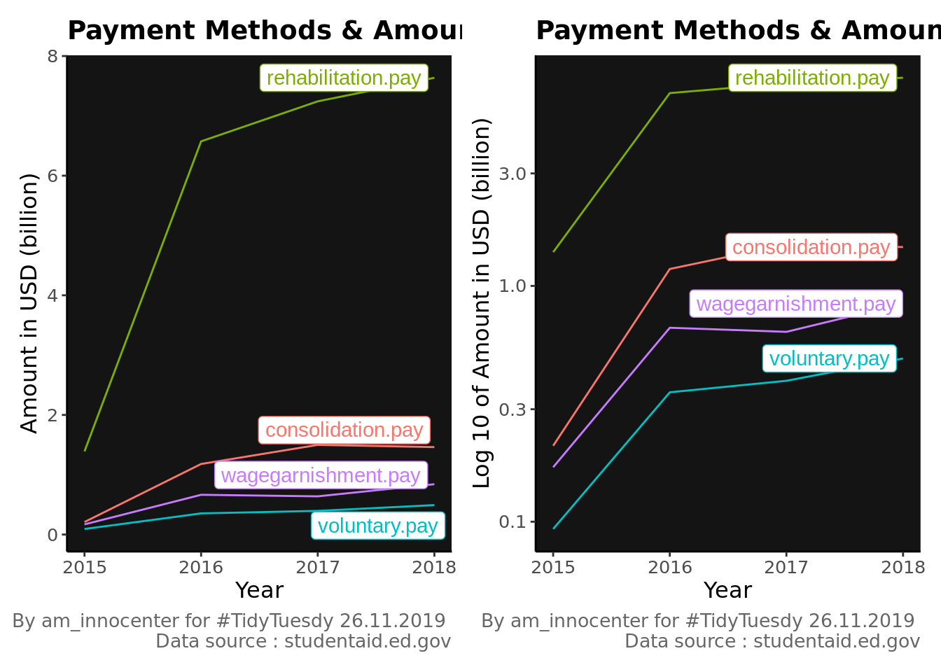

loans %>% 
  group_by(agency_name) %>% 
  summarise(Total.starting = sum(starting, na.rm=TRUE)/10^9, 
            Total.added = sum(added, na.rm = TRUE)/10^9,
            Total.repaid = sum(total, na.rm=TRUE)/10^9) %>% 
  arrange(desc(Total.starting)) %>% 
  filter(Total.starting > 30) %>% 
  ungroup() %>% 
  kableExtra::kable() %>% kableExtra::kable_styling()

agency_name	Total.starting	Total.added	Total.repaid
ConServe	109.05668	8.255166	3.3928101
Account Control Technology, Inc.	91.20824	8.254341	2.8479518
FMS Investment Corp	73.20214	8.254231	2.1526409
GC Services LP	70.19962	8.254341	1.8947032
Windham Professionals, Inc.	65.77404	8.254018	2.0332805
Immediate Credit Recovery, Inc.	50.69030	9.148463	1.1516027
Immediate Credit Recovery	40.24292	3.300990	0.8600955
FMS	37.40026	0.000000	0.9890860
Coast Professional, Inc.	36.48558	9.477421	1.1540227
GC Services	35.37406	0.000000	0.9639185
Coast Professional Inc	35.36888	7.604481	0.9776974
National Recoveries Inc	34.37731	7.211969	0.6891628
Action Financial Services	33.65348	6.487008	0.7403217
National Recoveries, Inc.	31.86218	8.850182	0.7083161